Part 21: The Magic Formula: Longitudinal Version
Brian Beckman, PhD
©Copyright February 2001
Driving a car is a classic problem in control. Here, we mean control in the technical sense of control theory, an established branch of engineering science (once again, I find http://www.britannica.com to have a very nice, brush-up article on that term). In a more-or-less continuous fashion, the driver compares desired direction, speed, and acceleration with actual direction, speed, and acceleration. The driver uses visual input to sense actual direction and speed; and uses visceral, inertial feedback-the butt sensor-for actual acceleration. When the actual differs too much from the desired, the driver applies throttle, brake, steering, and gear selection to change the actual. These inputs cause the tyres to react with the ground, which pushes back against the tyres, and through the suspension, pushes the body of the car and driver. Drivers in high-speed circumstances can also generate desired aerodynamic forces, as in slipstreaming, in the "slingshot pass," and in the Earnhardt TIP manoeuvre, where the driver "takes the air off" the spoiler of the car in front of him.
Tyres generate forces by sticking and sliding and everything in between. They transmit these forces to the wheels by elastic deformation. The elastic deformation is extremely complex and theoretical computation requires numerical solution of finite-element equations. However, despite fierce trade secrecy, industry and academia have reached apparent consensus in recent years on a formula that summarizes experimental and theoretical data. This so-called magic formula is not a solution to equations of motion-a solution in such a form is not feasible. It's just a convenient fitting of commonplace mathematical functions to data. It allows one to compute forces at a higher precision than something like RARS (see parts 16 and 19 of the Physics of Racing [PhOR]), but without integrating equations. Therefore, forces can be computed within a reasonable time, say in a real-time simulation program.
To understand the magic formula, we need first to define its inputs, which include slip. Slip is an indirect measure of the fraction of the contact patch that is sticking. It is frequently asserted in the literature that a tyre with no slip at all cannot create forces. It has taken me a very long time to accept this assertion. Why can I steer a tin-toy car with metal tyres on a hard surface like Formica? If there is any slip in such tyres, it is microscopic, yet there are sufficient forces to brake and steer, even if just a little. I finally caved in when I realized that the forces are minute, also. If there is any friction between the tyre and the surface, there MUST be slip, as it is defined below. Though to a very small degree, the Formica and the tiny contact patches of the tin tyres actually twist and stretch each other. The only way to eliminate slip completely is to eliminate GRIP completely. Any grip, and you will have slip.
There are two, slightly different flavours of the magic formula. The longitudinal one is the subject of this entire instalment of PhOR, and we cover the lateral one in the next instalment. Longitudinal slip is along the mean plane of the wheel and might also be called circumferential or tangential. It creates braking and accelerating forces. Lateral slip is our old friend grip angle [PhOR-10], and it generates cornering forces.
We write longitudinal slip as
 . It's defined by the actual angular velocity,
 , of a wheel plus tyre under braking or acceleration,
compared to the corresponding angular velocity of the same wheel plus tyre when
rolling freely. We write the free-rolling angular velocity as
, of a wheel plus tyre under braking or acceleration,
compared to the corresponding angular velocity of the same wheel plus tyre when
rolling freely. We write the free-rolling angular velocity as
 , where V is the current, instantaneous
velocity of the hub centreline of the wheel with respect to the ground, and Re
is the effective radius, a constant defined below. Since the dimensions of V
are length/time, and the dimensions of any radius are length, the ratio,
, has dimensions of inverse time. In
fact, it should be viewed as measuring radians per unit time, radians being the
natural, dimensionless measure of angular rotation. There are
, where V is the current, instantaneous
velocity of the hub centreline of the wheel with respect to the ground, and Re
is the effective radius, a constant defined below. Since the dimensions of V
are length/time, and the dimensions of any radius are length, the ratio,
, has dimensions of inverse time. In
fact, it should be viewed as measuring radians per unit time, radians being the
natural, dimensionless measure of angular rotation. There are
 radians in one rotation or one circumference of
a circle, just as the length of the circumference is
times the radius.
radians in one rotation or one circumference of
a circle, just as the length of the circumference is
times the radius.
Let's begin the discussion of longitudinal slip with a question. Consider a wheel-tyre combination with 13-inch radius or 26-inch diameter, say a 255-50/16 tyre on a 16-inch rim. The "50" in the tyre specification is the ratio of the sidewall height to the tread width, which is also written into the specification as 255, millimetres understood. We get a sidewall height of 50 percent of 255 mm, which is 5.02 inch. Therefore, the total, unloaded radius, half of the tread-to-tread diameter, is about 5 + 16/2 = 13 Inch. Now consider a rigid tyre of the same radius, made, say, of steel or of wood with an iron tread like old Western wagon wheels. The question is whether, given a certain constant hub velocity, pneumatic tyres spin faster than, slower than, or at the same speed as equivalent rigid tyres?
At first glance, one might say, "Well, faster, obviously. Since the pneumatic
tyre compresses radially under the weight of the car, its radius is actually smaller
than the unloaded radius at the point of contact, where it sticks and acquires linear
velocity equal in magnitude and opposite in direction to the hub velocity. Since
smaller wheels spin faster than larger ones at the same speed, the pneumatic tyre
spins faster than the equivalent rigid tyre of the same unloaded radius. Let the
unloaded, natural radius of the pneumatic tyre be R, also the radius of the
equivalent solid tyre. If the hub has velocity V, the solid tyre spins with
angular velocity
 . Since the loaded radius,
of the pneumatic tyre, Rl, is smaller than R, V/Rl,
the angular velocity of the loaded pneumatic tyre, must be larger than V/R."
. Since the loaded radius,
of the pneumatic tyre, Rl, is smaller than R, V/Rl,
the angular velocity of the loaded pneumatic tyre, must be larger than V/R."
This is partly correct. The pneumatic tyre-wheel combination does spin faster than a rigid wheel of the same unloaded radius, but it does not spin as fast as a rigid wheel of the same loaded radius, which is the height of the hub centre off the ground under load. The reason is that the tyre also compresses circumferentially or tangentially, setting up complex longitudinal twisting in the sidewall. The tangential speed of a particle of tread varies as the particle goes around the circumference of the tyre.
Let's mentally follow a piece of tread around as the wheel, not necessarily
the tyre, turns at a constant radial velocity,
 . Imagine a plug of yellow rubber embedded
in the tread, so that you could visually track it or photograph it with a movie
camera or strobe system as it moves around the circumference. The rubber of the
tread does not travel at constant speed, even though the wheel supporting the tyre
does. At the top of the tyre, the radius is almost exactly R, the unloaded
radius, so the tread moves with tangential velocity
. Imagine a plug of yellow rubber embedded
in the tread, so that you could visually track it or photograph it with a movie
camera or strobe system as it moves around the circumference. The rubber of the
tread does not travel at constant speed, even though the wheel supporting the tyre
does. At the top of the tyre, the radius is almost exactly R, the unloaded
radius, so the tread moves with tangential velocity
 . As the yellow plug rolls around and
approaches the contact patch from the front, it slows down in the bunched up area
at the leading edge of the contact patch-just forward of it. There is
a bunched-up area, because the tyre is made up of elastic material that gets squeezed
and stretched out of the contact patch and piles up ahead of the contact patch as
it rolls into it from the direction of the leading edge. Eventually, the plug enters
the patch, in the centre of which it must move at speed
. As the yellow plug rolls around and
approaches the contact patch from the front, it slows down in the bunched up area
at the leading edge of the contact patch-just forward of it. There is
a bunched-up area, because the tyre is made up of elastic material that gets squeezed
and stretched out of the contact patch and piles up ahead of the contact patch as
it rolls into it from the direction of the leading edge. Eventually, the plug enters
the patch, in the centre of which it must move at speed
 relative to the hub centre, that is,
backwards at a speed dictated by the loaded radius and the wheel velocity.
We've assumed that the plug is not slipping on the ground at the point where it
has speed
with respect to the hub. This means that
it has speed zero with respect to the ground at that point.
relative to the hub centre, that is,
backwards at a speed dictated by the loaded radius and the wheel velocity.
We've assumed that the plug is not slipping on the ground at the point where it
has speed
with respect to the hub. This means that
it has speed zero with respect to the ground at that point.
The average of the tangential velocities around the wheel defines the effective
radius, Re, as follows. Let
 measure the angular position, from 0 to
, around the wheel. Suppose we knew the tangential
velocity with respect to the hub centre, V(), at every
. We could easily measure this with our strobe light
and cameras. V() gives us the radius at every
angular position via the equation V()/
= R(), where
is the constant angular velocity of the
wheel. The average would be computed by the following integral:
measure the angular position, from 0 to
, around the wheel. Suppose we knew the tangential
velocity with respect to the hub centre, V(), at every
. We could easily measure this with our strobe light
and cameras. V() gives us the radius at every
angular position via the equation V()/
= R(), where
is the constant angular velocity of the
wheel. The average would be computed by the following integral:

Let's run some numbers. 10 mph is 14 feet/second or 176 inches/second. With an unloaded circumference of
 inch/revolution, we get 176/= 2.154 revs per second, or 129 RPM for each 10 MPH.
Under ordinary circumstances, the effective radius will be no more than a few percent
less than then the unloaded radius, and the RPMs should be, then, a few percent
more than 129 RPM per 10 MPH. At 100 MPH, the tyre is under considerable stress
and spins at something over 1,300 RPM.
inch/revolution, we get 176/= 2.154 revs per second, or 129 RPM for each 10 MPH.
Under ordinary circumstances, the effective radius will be no more than a few percent
less than then the unloaded radius, and the RPMs should be, then, a few percent
more than 129 RPM per 10 MPH. At 100 MPH, the tyre is under considerable stress
and spins at something over 1,300 RPM.
Now we're in a position to define longitudinal slip, written
. We want a quantity that vanishes when the wheel rolls
at constant speed, increases when the wheel accelerates the car by pulling the contact
patch backwards, and decreases below zero when then wheel brakes the car by pushing
the contact patch forward. Under acceleration, the wheel and tyre combination will
tend to spin a little faster than it would do while free rolling. We already know
that, for a given V, the free-rolling angular velocity is
, by definition. The actual angular velocity,
, then, is higher under acceleration. So, if we know
V,
, and the constant Re, then we can
define the longitudinal slip as the ratio, minus 1, so that it's zero under free-rolling
conditions:
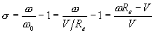
Just looking at this formula, a free-rolling wheel has
 ,
= 0 a locked-up wheel under braking has
= 0,
= -1 and an accelerating wheel has a positive
of any value.
,
= 0 a locked-up wheel under braking has
= 0,
= -1 and an accelerating wheel has a positive
of any value.
The magic formula yields the longitudinal force, in Newtons, given some constants
and dynamic inputs. The formula takes eleven empirical numbers that characterize
a particular tyre {b0, b1...b10}.
The dynamic parameters are Fz, or weight, in KiloNewtons
on the tyre, and the instantaneous slip,
. The eleven numbers are measured for each tyre. We
borrow an example from Motor Vehicle Dynamics by Giancarlo Genta. On page
528, he offers the following numbers for a car that appears to be a Ferrari 308
or 328, to which I have added dimensions:
|
|
Though the majority of these values are zero for the tyres on this car, it is by no means always the case. In fact, the 'large-saloon' example just before the (alleged) Ferrari in Genta's book has no zeros.
We build up the magic formula in stages. The first helper quantity is µp = b1Fz + b2. This is an estimate of the peak, longitudinal coefficient of friction, fitted as a linear function of weight (see Part 7 of PhORs). From this definition, we begin to see what's going with the dimensions. A typical, streetable sports car might weigh in at 3,000 lbs, which is about 3,000 / 2.2 = 1,500 * 0.9 = 1,350 kg, which is about 1,350 * 9.8 = 13,200 Newtons, or 13.2 KiloNewtons (look, ma, no calculator!). Let's assume each tyre gets a quarter of that to start off with, or 3.3 KN. b1 multiplies that number to give us something with dimensions of KiloNewton/MegaNewton, which we write simply as 1/Kilo (inventing units on-the-fly, one Mega = 1 Kilo squared). b2 has the same dimensions, so it's kosher to add it in, yielding µp = 1688 / Kilo in this case. The next step is the helper D = µpFz, which will be in Newtons. We now see the reason for the 1/Kilo unit. In our case, we get about D = (1700 - 12) * 3.3 = 5610 - 40 = 5570 N. The important point is that D is linear in Fz, so µp acts, mathematically, like a coefficient of friction, as promised. b2 is a pretty direct measurement of stickiness, times 1,000 for convenience. This model tyre has a coefficient of friction of almost 1.7! Not my data, man.
The next step is to compute the product of a new helper, B, times b0 and the aforecomputed D. The magicians who created the formula tell us that Bb0D = (b3Fz2 + b4Fz) exp(-b5Fz). This slurps up a few more of the magical eleven empirical numbers, and a pattern emerges. These bi numbers serve as coefficients in polynomial expressions over Fz. So, b5Fz is dimensionless, as must be the argument of the exponential function. b3Fz2 + b4Fz has dimensions of Newtons, as does the entire product. Therefore, B must be dimensionless. We need B in the next step, so let's solve for it now:
 ,
,
Where we've been able symbolically to divide out one factor of Fz, convenient especially for numerical computation, where overflow is an ever-present hazard. Continuing with our numerical sample, b3Fz + b4 = 229 / Kilo, the exponential is unity, and the numerator is

yielding B = 229 / 2786 = 0.0822. Most importantly, B depends only weakly on Fz. In the sample case, not at all, because b1 = b3 = b5 = 0, but there are lots of other ways to characterize the algebraic dependence of B on Fz.
The next step is to account for the longitudinal slip with another helper, S = (100+ b9Fz + b10);
in our sample case, this reduces to just S = 100.
Only one more helper is needed, and that's E = (b6Fz2 + b7Fz + b8), very straightforward. The final formula is

Once again, don't try to find any physics in here: it's just a convenient formula
that fits the data reasonably well. Plugging in numbers for
= 0, because that's an easy sanity check to do in our heads,
we see immediately the result is zero. Let's try S = 10, ten percent
slip. SB = 0.822, tan-1(0.822) = 0.688, E = -10,
so the argument of the outer arctangent is SB - 10 * (-0.266) = SB + 2.66 = 3.48,
tan-1(3.48) = 1.29, 1.29 b0 = 2.13,
sin(2.13) = 0.848, and, finally, D * 0.848 = 4720 Newtons.
Lots of longitudinal force for a 3,300 N vertical load!
Let's plot the whole formula:
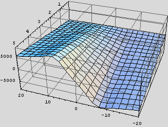
The horizontal axis measures S = 100, which is really just slip in percent.
The deep axis, going into the page, measures Fz from 5 KN, nearest
us, to zero in the back. The vertical axis measures the result of applying the formula
to our model tyre, so it's longitudinal force-force of launching or braking. Notice
that for a load of 5 KN, the model tyre can generate almost 8 KN of force. Very
sticky tyre, as we've already noticed! Also notice that the generated force peaks
at around
= 0.08, or 8 percent. The peak would be something one could
definitely feel in the driver's seat. Overcooking the throttle or brakes would produce
a palpable reduction in g-forces as the tyres start letting go. Worse than that,
increasing braking or throttle beyond the peak leads to reduced grip. This is an
instability area, where increasing slip leads to decreasing grip.
Finally, note that the function behaves roughly linearly with Fz, showing that it acts like a Newtonian coefficient of friction, albeit a different one for each value of slip.